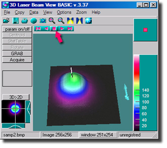
Fig.1. The Main Form, 3D and 3D windows, Animation control toolbar.
Installation / de-installation is automatic, just run *.msi file from CD or downloaded for performing desired action.
Main Form
Start the program from Start menu or desktop icon. The laser beam sample image will appear. The image file under processing is shown in StatusBar first panel (see Fig.1). The Main Form window is shown in Fig.1. The StatusBar indicates original image size as height and width in pixels, and 3D window pixel size. The 3D window size panel is clickable to provide you with possibility to change the 3D picture size. The 3D window is animated (rotated around Z axis) by default. You can stop the animation by pressing the "pause" button at the Animation Control Tool as shown in Fig.1. To run rotation again clock wise or anticlock wise, click "Run" triangle at the Animation Control Tool. The Main Window supports 2 basic modes: 3D maximized and 2D maximized. To toggle between the modes use "3D to 2D" button at left down portion of the main form.
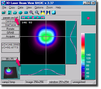
Fig.2. 2D View Mode, 1D beam profile plots, Gaussian fits.
You can switch between 3D mode and 2D mode by "3D to 2D" button as shown in Fig.2. This will maximize 2D sub-window. Enable beam parameters calculations mode as shown in Fig.2, upper arrow. Use parameter buttons to calculate specific parameter. The buttons are enabled in calculation mode (see Fig.2, left side button group). Press "Centroid" button in this group (see Fig.3). This will calculate centroid position as shown in main form at left side (see xC and yC, values are given in pixel units).
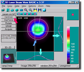
Fig.3. True ellipse and Gaussian fits. Beam parameters and statistics.
"StatTable" button will perform main statistics calculation and bring you the result form. The ellipse will be calculated and drawn around the beam. The ellipse is found as true least square fit in 2D for the beam at 13% intensity level. The resulting ellipse is shown as white ellipse line (Fig.3, blue arrow). The Gaussian fits are calculated for both vertical and horizontal intersection (Fig.3 red line marked by the cyan arrow). The fit profile is drawn together with measured profile (Fig.3, red and white lines respectively). The Gaussian fit is calculated as least square to all points in profile. We note here that we apply quite sophisticated ellipse and Gaussian fits implemented as true Least square incremental search algorithm as compared to most of the software packages that utilize simplified less accurate algorithms.
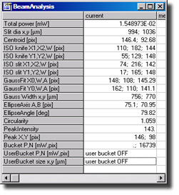
Fig.4. Diameter calculation. Beam parameters with Gaussian fitting and ISO.
Beam parameter and statistics table
The results of the statistical beam parameter calculation is shown in Fig.4. The laser beam diameter measurement is shown in both pixel and micron units. The most reliable diameter measurement for single mode beams is given by Gaussian width. For complicated beams you can use ISO slit and knife diameters as defined by ISO. All diameters are calculated separately in X and Y directions.
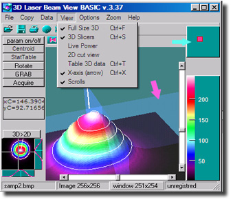
Fig.5. 3D visualization options: Interactive
intersection planes, 3D Light position, 3D contour lines.
3D visualization options
Return to
3D mode by "3D to 2D" button. Use Menu>Data>AutoscaleZ to scale
Z into whole color palette scale. See change of the 3D and 2D images.
Use menu>View> to try following options:
3D slicers ON/OFF
X-axis arrow ON/OFF
Scrolls ON/OFF
Contour ON/OFF
Slicers
(orthogonal intersection planes) are the semitransparent interactive cut
planes used to obtain orthogonal cut profiles. In Fig.5, the magenta arrow
indicates the area to pick up and move the plane with mouse. While you
pick up plane and move it you will see "Focus" white lines at
the plane corners.
You can adjust the light position relative to surface using Light position
tool (Fig.5, cyan arrow). Click and drag Mouse operation anywhere within
the light tool to change light position relative to surface origin.
If you need for example to see noise level of your imager background,
you can adjust light position to be inclined and activate specular 3D
mode. This will provide you with great enhancement of the surface features.
In Fig.6 we show the offset noise at low intensity level.
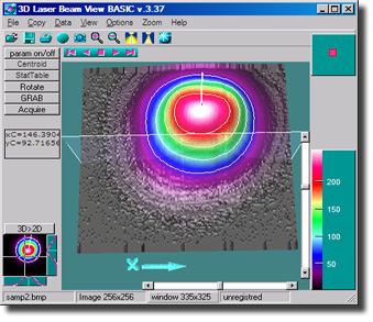
Fig.6. 3D visualization of laser beam. Intersection Planes are shown. Light is set to be inclined for better observation of the noise.
Menu>Options>Reflections option toggle surface specular or reflective. Specular surface representation helps you to see fine structure of the surface.
You can use Zoom Tools to zoom surface in and out. Zoom can be used either from menu or by magnifier buttons of the main toolbar.
Go Menu>View>2D cut View to initiate 2D cut form.
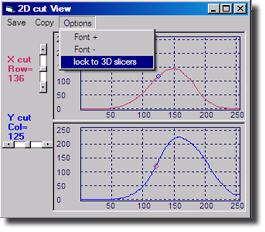
Fig.7. 2D plot of the 1D intersections between laser beam surface and cut planes. Laser beam profiling is achieved by moving orthogonal X and Y planes in 3D window or by setting the plane position within 2D view form.
Detailed intersection plot form.
Cut View.
The form is called from Menu>View.
You can use this 2D cur Viewer to see detail of the laser beam profiles
at the slicer position in both X and Y directions.
You can use "lock to 3D slicers" option
to link movement of the slider within 2D with 3D cut plane position.